CHAPTER - 9
FINITE ELEMENT ANALYSIS
9.1 INTRODUCTION
9.2 FINITE ELEMENT DISPLACEMENT ANALYSIS
9.3 TWO-DIMENSIONAL HEAT CONDUCTION IN COMPOSITE LAMINATES
9.4 TWO DIMENSIONAL HYGROTHERMAL DIFFUSION IN COMPOSITES
9.5 Bending and Vibration of laminated Composite Plates and Shells
9.6 BIBLIOGRAPHY
9.7 EXERCISES
The solution of a real life problem involving an arbitrary plate geometry and complicated loading and boundary conditions cannot be easily realized using the analytical methods discussed in chapters 7 and 8. A numerical analysis technique, especially the finite element analysis method, is suited most to tackle such problems. Further, unlike the metallic structure, the design of a composite structure is, in most cases, preceded by the design of the composite material with which the structure is made. The hygrothermal environment, the temperature dependence of thermo-mechanical properties, the anisotropy, the stacking sequence and several other parameters involving material, geometry, loading and service conditions endorse the need for the application of the finite element analysis techniques in composite materials and structures.
The finite element
method is essentially a piecewise application of a variational method. The
finite element formulation is, therefore commonly, based on the conventional
Rayleigh-Ritz method (Ritz method) and the Galerkin method (weighted residual
method). In the Rayleigh-Ritz method we construct a functional that express the
total potential energy ![]() of the system in terms of nodal variables d1. The
problem is solved using the stationary-functional conditions
of the system in terms of nodal variables d1. The
problem is solved using the stationary-functional conditions
![]() . In the case of the Galerkin method, the functional for the
residual R is formed using differential equations of the physical problem. The
problem is solved by setting the weighted averages of the residual R to zero,
i.e.,
. In the case of the Galerkin method, the functional for the
residual R is formed using differential equations of the physical problem. The
problem is solved by setting the weighted averages of the residual R to zero,
i.e., ![]() , where W1 are the weight functions. The Galerkin
method find applications in several non-structural physical problems. In
structural mechanics, both the Rayleigh-Ritz method and the Galerkin method
yield identical results, when both use the same field variables.
, where W1 are the weight functions. The Galerkin
method find applications in several non-structural physical problems. In
structural mechanics, both the Rayleigh-Ritz method and the Galerkin method
yield identical results, when both use the same field variables.
9.2 FINITE ELEMENT DISPLACEMENT ANALYSIS
The displacements {u} within an element are usually expressed as
{u} = [N] {de} (9.1)
where [N] is the shape function
and {de} is the element nodal displacements with respect to the local
axis. The strains {![]() } in an element are defined in terms of the displacements as
} in an element are defined in terms of the displacements as
![]() (9.2)
(9.2)
where [Δ] is an appropriate differential operator. Now, combining Eqs. 9.1 and 9.2, the relations between the strains and nodal displacements are obtained as
![]() (9.3)
(9.3)
where
![]() (9.4)
(9.4)
The stresses and strains in an element are defined as
![]() (9.5)
(9.5)
where [Q] are the elastic stiffnesses. Hence the stress-nodal displacement relations are derived as
![]() (9.6)
(9.6)
The total potential of an element is first computed to apply the Rayleigh-Ritz variational approach. This is equal to the sum of the strain energy developed in the element and the work done by the applied forces on the surface of the element. The work done by the body forces within the element is neglected in the present case.
Thus, the total potential of the element is given by
![]() (9.7)
(9.7)
where {q} are the surface tractions.
Combining Eqs. 9.1, 9.3, 9.6 and 9.7, we obtain
![]() (9.8)
(9.8)
Applying the principle of
Minimum Potential Energy i.e., ![]() yields
yields
[Ke] {de} ={Pe} (9.9)
where [Ke] is the element stiffness matrix and {Pe} are the element nodal forces. These are defined as
![]()
and ![]() (9.10)
(9.10)
Transformation of Eq. (9.9) from the local axes to the global axes and proper assembly of terms over all elements will lead to a set of equilibrium equations for the complete structure, as given by
![]() (9.11)
(9.11)
where [K], {d}and {P} correspond to the global axes.
When the Galerkin weighed residual approach is employed, the residual equation is expressed in the form
![]() (9.12)
(9.12)
where
![]() are the equilibrium equations, and the shape functions [N]
are the weight functions. Applying the Green-Gauss theorem to Eq. 9.12 and
expanding and then employing Eqs. 9.1 through 9.4, one obtains
are the equilibrium equations, and the shape functions [N]
are the weight functions. Applying the Green-Gauss theorem to Eq. 9.12 and
expanding and then employing Eqs. 9.1 through 9.4, one obtains
![]() (9.13)
(9.13)
after eliminating the non-essential boundary conditions. Equations. 9.13 can be written in the form as that given by Eqs. 9.9, where [Ke] and {Pe} are defined in Eqs. 9.10.
9.3 TWO-DIMENSIONAL HEAT CONDUCTION IN COMPOSITE LAMINATES
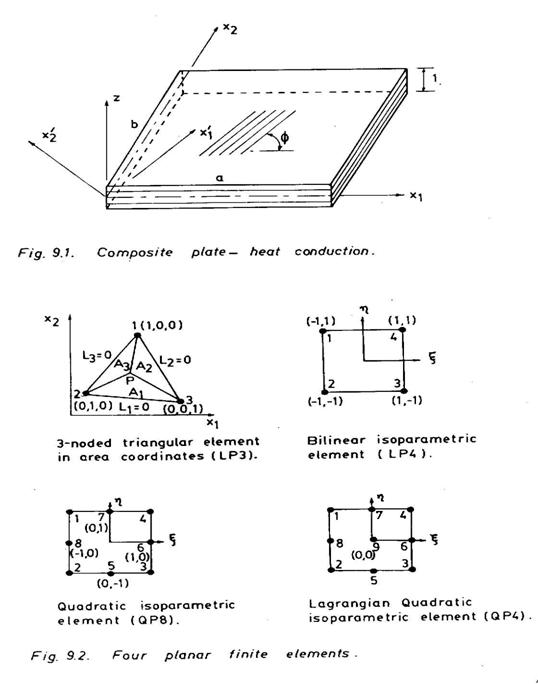
The axes system of a rectangular laminated composite plate is presented in Fig. 9.1. It is assumed that the temperature varies along the x1x2 plane, but remains constant through the thickness of the plate. The two-dimensional heat conduction equation for the composite plate then assumes the form
![]() (9.14)
(9.14)
where K11 and K22 are the laminate conductivities, T is the temperature field, ρ is the mass per unit area of the plate, c is the heat capacity, t is the time and the associated boundary conditions are
![]() (9.15)
(9.15)
with 11 and 12
are direction cosines and ![]() is the boundary heat flux.
is the boundary heat flux.
The Galerkin finite element method is now employed. The residual equation for the composite plate takes the form
![]() (9.16)
(9.16)
where [N] is the shape function matrix and a dot denotes differentiation with respect to time.
Fig. 9.1
Integration of Eq. 9.16 yields
 (9.17)
Expressing the temperature variables as
{T} = [N] {Te}
and substituting in Eq. 9.17 one obtains
 (9.18)
Equation 9.18 finally reduces to
![]() (9.19)
(9.19)
where
![]() (9.20)
(9.20)
![]() (9.21)
(9.21)
and
![]() (9.22)
(9.22)
Note that the conductivity matrix for the laminate is given as
 (9.23)
and
 (9.24)
where Ni is the shape function of an element with p nodes.
Consider a laminated composite plate (Fig. 9.1), where each side is of length a i.e., a = b. The temperature specified on the boundaries are
x1=0,a and x2 = 0 : T = 273k
x2 = a : T = 773k
The laminate conductivities are
K11 = 10.03 W/cm K and K22 = 1.71 W/cm K
The analytical solution to the problem is found to be
![]() (9.25)
(9.25)
where
![]()
The problem is also analysed using the Galerkin finite element approach. Four elements (Fig. 9.2) are employed.
Fig. 9.2
The shape functions are given as follows:
3-noded triangular element in area coordinates (LP3):
Ni = Ai/A, i = 1,2,3 (9.26)
4-noded bilinear isoparametric element (LP4) :
![]() i = 1,2,3,4 (9.27)
i = 1,2,3,4 (9.27)
8-noded quadratic isoparametric element (QP8):
![]()
![]()
![]() i = 5,7 (9.28)
i = 5,7 (9.28)
![]() i = 6,8
i = 6,8
9-noded quadratic isoparametric element (QP9)
![]()
![]()
![]() i = 5,7 (9.29)
i = 5,7 (9.29)
![]() i = 6, 8
i = 6, 8
![]() i = 9
i = 9
The transformation
of coordinates from the Cartesian system x1x2 to the
isoparametric system ![]() is necessary for the use of isoparametric planar elements
(Fig. 9.2). For example, in the isoparametric coordinates, Eq. 9.20 assumes the
form
is necessary for the use of isoparametric planar elements
(Fig. 9.2). For example, in the isoparametric coordinates, Eq. 9.20 assumes the
form
![]() (9.30)
(9.30)
in which the Jacobian J arises due to the change of coordinates. The matrix [B] is also expressed as
 (9.31)
where the Jacobian matrix is given by
 (9.32)
The comparision between the analytical solution using Eq. 9.25 and the finite element solution employing four planar finite elements with meshes corresponding to nearly identical degrees of freedom, are presented in Table 9.1. The results depict the steady state temperature at four locations along the line x1 = a/2. The Lagrangian QP9 element exhibits close proximity to analytical results.
The steady state temperature distribution in two antisymmetrically laminated (00/300/00/300) GT75/Nickel and SiC/6061 Al metal matrix composite plates are plotted in Figs. 9.3 and 9.4. The laminate conductivities are derived using Eq. 4.45 (replace 'd' with ' k' ) and Eq. 11c of Table 4.1, where Kf = 10.03 W/cmK, Km = 0.62 W/cmK and Vf = 0.5 for the GT75/Nickel composite and Kf = 0.16 W/cmK, Km = 1.71 W/cmK and Vf =0.5 for the SiC/6061 Al composite.
Fig. 9.3
Fig. 9.4
Table 9.1 : Comparison of results
Locations Element FEM Analytical %error
X1 = a/2 LP3 289.27 +1.12
X2 = a/2 LP4 284.64 -0.49
QP8 286.59 286.06 +0.18
QP8 286.64 +0.20
x1 = a/2 LP3 313.39 +1.20
x2 = 5a/8 LP4 304.26 -1.74
QP8 312.64 309.66 +0.96
QP9 309.67 +0.00
x1 = a/2 LP3 372.19 +1.30
x2 = 3a/4 LP4 359.30 -2.18
QP8 361.53 367.32 -1.58
QP9 364.53 -0.76
x1 = a/2 LP3 508.31 +0.12
x2 = 7a/8 LP4 506.64 -0.20
QP8 507.85 507.68 -0.03
QP9 507.67 -0.00
Mesh size: LP3: 16x16, LP4: 8x8, QP8: 4x4, QP9: 4x4
9.4 TWO DIMENSIONAL HYGROTHERMAL DIFFUSION IN COMPOSITES
Here we discuss the finite element analysis procedure where the spectral distribution of temperature and moisture are determined simultaneously. This is essentially an uncoupled problem. The temperature field is first evaluated using the procedure discussed in section 9.3. The diffusion of moisture is then analysed with the updated material diffusivity data, which are dependent on temperature. The finite element formultation of moisture diffusion is identical to that of heat conduction. The temperature dependent two-dimensional moisture diffusion equation is given by
d11C,11 + d22 C,22 = C,t (9.33)
where d11 and d22 are the moisture diffusivities and are dependent on temperature and C is the moisture concentration at a time t.
The boundary conditions are
![]() (9.34)
(9.34)
where ![]() is the boundary moisture flux.
is the boundary moisture flux.
Applying the Galerkin finite element approach, the residual equation assumes the form
![]() (9.35)
(9.35)
The moisture field within the element is assumed as
{C} =[N] {Ce} (9.36)
where [N] is the shape function matrix and {Ce} are the nodal moisture concentration vector for the element. Expanding Eq. 9.35 and substituting Eq. 9.36 in Eq. 9.35 yield, for the element
![]() (9.37)
(9.37)
where
![]() (9.38)
(9.38)
![]() (9.39)
(9.39)
![]() (9.40)
(9.40)
The diffusivity matrix [d] is given by
 (9.41)
Consider the diffusion of moisture through a single fibre polymer composite model (Vf = 0.385) as shown in Fig. 9.5. The composite model consists of a carbon fibre embedded in an epoxy matrix. The fibre is assumed to be impermaeable to moisture. The matrix is initially saturated with 2% moisture concentration i.e., Ci = 0.002. The initial temperature of the composite is specified as Ti = 300K. The outside opposite faces of the composite model are now exposed to zero moisture concentration level (Cs = 0) and a sudden temperature rise of 573K (Ts = 573K). Only a quarter of the composite model is considered for the finite element analysis. The boundary conditions considered are given by for the fibre:
![]()
for the matrix:
![]()
x1 = 0 : CS = 0, TS = 573K
x2 = 0, a:
![]()
and for the fibre-matrix
interface : ![]()
The relevant hygrothermal material parameters are presented in Table 9.2. The diffusivity dm of the matrix is assumed to be
Table 9.2: Hygrothermal parameters for fibre and matrix
Material Conductivity, k Coefficient of thermal d0 A
W/cm K expansion α x 10-6/K cm2/sec K
Fibre 10.03 -1.1 0 -
Matrix 0.0072 22.5 1.637 5116
Temperature dependent as given by
dm = d0 e-A/T (9.42)
where d0 is the diffusivity at 300 K.
The distribution of transient moisture and temperature along the x1 axis are plotted in Fig. 9.5. Eight noded isoparametric elements (QP8) are employed for the analysis. An implicit time integration scheme, based on the Galerkin method (µ = 2/3), is employed to determine the transient temperature and moisture field. The temperature is observed to be almost saturated at 573 K through the fibre and the matrix at t = 1 sec., but the moisture diffuses through the matrix at a much slower rate.
Fig. 9.5
9.5 Bending and Vibration of laminated Composite Plates and Shells
Consider a doubly curved laminated composite shallow shell of thickness h and principal radii of curvature R11, R22 and R12 approach infinity. The shell laminate consists of n number of arbitrarily oriented laminae. The lamina behaviour accounts for the first order transverse shear deformation of the Reissner-Mindlin type. This permits the use of the present analysis to solve composite sandwich plates and shells as well, when one or more plies assume the elastic properties of core materials.
Fig. 9.6
The stress resultants on a composite shell element are shown in Fig. 9.7 and are expressed in terms of mid-plane strains and curvature as
 (9.43)
where Aij, Bij, Dij, Sij,Kij are defined in Eqs. 8.3 through 8.5. Also, for each lamina
![]()
![]() (9.44)
(9.44)
![]()
where ' refers to the principal material axes x1'x2'.
Fig. 9.7
Assume an eight-noded
quadratic isoparametric doubly curved shell element (Fig.9.8), where the
mid-plane displacements i.e., degrees of freedom per node are defined as three
translational displacements ![]() and two bending rotations
and two bending rotations
![]() (see section 8.3). These are expressed in terms of their
nodal values by the element shape functions and are given by
(see section 8.3). These are expressed in terms of their
nodal values by the element shape functions and are given by
![]() (9.45)
(9.45)
where the shape functions are defined in Eq. 9.28.
Fig. 9.8
The strain-displacement relations based on an improved shallow shell theory using the modified Donnell's approximations, are expressed as
 (9.46)
where
![]() correspond to the mid-surface strains an d{K} are the
curvatures, and are given by
correspond to the mid-surface strains an d{K} are the
curvatures, and are given by
 (9.47)
and
![]() (9.48)
(9.48)
The strain nodal displacement relations for the element is given by
![]() (9.49)
(9.49)
where

and the matrix [B] is obtained substituting Eq. 9.45 in Eqs. 9.46 through 9.49 and is expressed as

(9.50)
The element stiffness matrix is given by
![]() (9.51)
(9.51)
Note that the stiffness matrix [D] in the above relation is expressed as
 (9.52)
as given in Eq. 9.43.
The element mass matrix is expressed as
![]() (9.53)
(9.53)
where
 (9.54)
and
 (9.55)
with
 and
and
 (9.56)
Here ρ is the mass density.
The element level load vector due to transverse load {q} per unit area is obtained
![]() (9.57)
(9.57)
The stiffness matrix [Ke]
and [Me] are evaluated first by expressing the integrals in the local
isoparametric coordinates ![]() and
and ![]() of the element and then performing numerical integration
employing the 2x2 Gauss quadrature. The element matrices are assembled after
performing appropriate transformations due to the curved shell surface to obtain
the global matrices [K] and [M]. Thus, one obtains for the static case
of the element and then performing numerical integration
employing the 2x2 Gauss quadrature. The element matrices are assembled after
performing appropriate transformations due to the curved shell surface to obtain
the global matrices [K] and [M]. Thus, one obtains for the static case
[K] {d} = {P} (9.58)
and for the free vibration case
![]() (9.59)
(9.59)
Table 9.2 shows the
results in non-dimensional form ![]() and
and ![]() at the centre (x1 = a/2, x2 = a/2) of a
simply supported laminated [(00/900)4/00]
paraboloid of revolution shell (Fig. 9.9) with
at the centre (x1 = a/2, x2 = a/2) of a
simply supported laminated [(00/900)4/00]
paraboloid of revolution shell (Fig. 9.9) with
![]() when it is acted upon by a uniformly distributed transverse
load q0. The shear of deformation of the laminae is, however,
neglected here. The convergence of results seems to be reasonably good.
when it is acted upon by a uniformly distributed transverse
load q0. The shear of deformation of the laminae is, however,
neglected here. The convergence of results seems to be reasonably good.
Fig. 9.9
Table 9.2 : Non-Dimensional displacement and force and moment resultants
Mesh
size
![]()
![]()
![]()
2 x 2 2.839 3.063 5.313
3 x 3 2.771 3.032 5.277
4 x 4 2.746 3.021 5.259
6 x 6 2.729 3.013 5.245
8 x 8 2.722 3.009 5.240
The non-dimensional
fundamental frequencies ![]() for simply supported laminated composite spherical shells (R11
= R22 = R, R12 = 0) with
for simply supported laminated composite spherical shells (R11
= R22 = R, R12 = 0) with
![]() = 25
= 25 ![]() ,
, ![]() =
= ![]() = 0.5
= 0.5 ![]() , a/b = 1, a/h =100 are presented in Table 9.3. A 6 x 6 mesh
is used to discretize the shell. Note that R11 = R22 =
, a/b = 1, a/h =100 are presented in Table 9.3. A 6 x 6 mesh
is used to discretize the shell. Note that R11 = R22 =
![]() corresponds to a flat plate.
corresponds to a flat plate.
Table 9.3 : Non-dimensional fundamental frequencies
h / R11 00/900 00/900/00
1/300 45.801 47.035
1/400 35.126 36.890
1/500 28.778 30.963
1/1000 16.706 20.356
Plate 9.689 15.192
The frequencies are found to be comparatively lower for the (00/900) laminate due to the bending-stretching coupling effect. Further, as the curvature reduces, the frequency comes down. The dynamic stiffness is the lowest for the flat plate. The coupling effect is more pronounced in the case of a plate.
1. R. D. Cook, D.S. Malkus and M.E. Plesha, Concepts and Applications of Finite Element Analysis, Wiley, NY, 1989.
2. K.J. Bathe, Finite Element Procedures in Engineering Analysis Preintice-Hall of India, New Delhi, 1990.
3. O.C. Zienkiewicz and R.L. Taylor, The Finite Element Method, Vol.2, McGraw-Hill Bood Co., NY, 1991.
4. S.S. Rao, The Finite Element Method in Engineering, Peergamon, NY, 1989.
5. J.N. Reddy, An Introduction to Finite Element Method, McGraw Hill, NY.,1992.
6. W.Jost, Diffusion in Solids, Liquids and Gases, Academic Press, 1960.
7. J. Crank, Mathematical Theory of Diffusion, Oxford Press, London, 1975.
8. J.S. Carslaw and J.C. Jaegar, Conduction of Heat in Solids, Clarendon, Oxford, 1959.
9. K.S. Sai Ram and P.K. Sinha, Hygrothermal Effects on the Bending Characteristics of Laminated Composite Plates, Computers and Structures, 40, 1991, p. 1009.
10. K.S Sai Ram and P.K. Sinha, Hygrothermal Effects on the Free Vibration of Laminated Composite Plates, J. Sound and Vibration, 158, 1992, p. 133.
11. K.S Sai Ram and P.K. Sinha, Hygrothermal Effects on the Buckling of Laminated Composite Plates, Int. J. Composite Structures, 21, 1992, p.233.
12. A. Dey, J.N. Bandyopadhyay and P.K. Sinha, Finite Element Analysis of Laminated Composite Paraboloid of Revolution Shells, Computers and Structures, 44, 192, p. 675.
13. A. Dey, J.N. Bandyopadhyay and P.K. Sinha, Finite Element Analysis of Laminated Composite Conoidal Shell Structures, Computers and Structures, 43, 1992, p. 469.
14. K.S Sai Ram and P.K. Sinha, Hygrothermal Bending of Laminaated Composite Plates with a Cutout, Computers and Structures, 43, 1992, p. 1105.
15. K.S Sai Ram and P.K. Sinha, Hygrothermal Effects on Vibration and Buckling of Laminated Plates with a Cutout, AIAAJ, 30, 1992, p. 2353.
16. N. Mukherfee and P.K. Sinha, A Finite Element Analysis of Inplane Thermostructural Behaviour of Composite Plates, J. Reinforced Plastics and Composites, 12, 1993, p. 1026.
17. N. Mukherfee and P.K. Sinha, A Finite Element Analysis of Thermostructural Bending Behaviour of Composite Plates, J. Reinforced Plastics and Composites, 12, 1993, p. 1221.
18. N. Mukherfee and P.K. Sinha, A Comparative Finite Element Heat Conduction Analysis of Laminated Composite Plates, Computers and Structures, 52, 1994, p. 505.
19. N. Mukherfee and P.K. Sinha, Three Dimensional Thermostructural Analysis of Multidirectiional Fibrous Composite Plates, Int. J. Composite Structures, 28, 1994, p. 333.
20. A. Dey, J.N. Bandyopadhyay and P.K. Sinha, Behaviour of Paraboloid of Revolution Shell Using Cross-ply and Antisymmetric Angle-ply Laminates, Computers and Structures, 52, 1994, p. 1301.
21. D. Chakravorty, J.N. Bandyopadhyay and P.K. Sinha, Finite Element Free Vibration Analysis of Point Supported Laminated Composite Cylindrical Shells, J. Sound and Vibrations, 18, 1995, p. 43.
22. D.K. Maiti and P.K. Sinha, Bending and Free Vibration of Shear Deformable Laminated Composite Beams by Finite Element Method, Int. J. Composite Structures, 29, 1994, p. 421.
23. T. V. R. Choudary, S. Parthan and P.K. Sinha, Finite Element Flutter Analysis of Laminated Composited Panels, Computers and Structures, 53, 1994, p. 245.
24. D. Chakravorty, J.N. Bandyopadhyay and P.K. Sinha, Free Vibration Analysis of Point Supported Laminated Composite Doubly Curved Shells – A Finite Element Approach, Computers and Structures, 54, 1995, p. 191.
25. P.K. Sinha and S. Parthan (Eds.), Computational Structural Mechanics, Applied Publishers Ltd., New Delhi, 1994.