The formulae presented in this chapter are based on the classical bending theory of thin composite plates. The small deflection bending theory for a thin laminate composite beam is developed based on Bernoulli's assumptions for bending of an isotropic thin beam. The development of the classical bending theory for a thin laminated composite plate follows Kirchhoff's assumptions for the bending of an isotropic plate. Kirchhoff's main suppositions are as follows:

The material behaviour is linear and elastic.
The plate is initially flat.
The thickness of the plate is small compared to other dimensions.
The translational displacements (and w) are small compared to the plate thickness, and the rotational displacements () are very small compared to unity.
The normals to the undeformed middle plane are assumed to remain straight, normal and inextensional during the deformation so that transverse normal and shear strains () are neglected in deriving the plate kinematic relations.
The transverse normal stresses are assumed to be small compared with other normal stress components . So that they may be neglected in the constitutive relations.

The relations developed earlier in sections 6.12 and 6.13 are essentially based on the above Kirchhoff's basic assumptions. Some of these relations will be utilized in the present chapter to derive the governing equations for thin composite plates. It may be noted that Kirchhoff's assumptions are merely an extension of Bernoulli's from one-dimensional beam to two-dimensional plate problems. Hence a classical plate bending theory so developed can be reduced to a classical beam bending theory. Here, also, the governing plate equations are derived first, and the beam equations are subsequently obtained from the plate equations.

7.2 THIN LAMINATED PLATE THEORY

Consider, a rectangular, thin laminated composite plate of length a, width b and thickness h as shown in Fig.7.1. The plate consists of a laminate having n number of laminae with different materials, fibre orientations and thicknesses. The plate is subjected to surface loads q's and m's per unit area of the plate as well as edge loads per unit length. The expansional strains, which may be caused due to moisture and temperature, are also included. Note that and w are mid-plane displacement components. It is assumed that Kirchhoff's assumptions for the small deflection bending theory of a thin plate are valid in the present case. One of these assumptions is related to transverse strains which are neglected in derivation of plate kinematic relations i.e., stress-strain relations.

Considering the dynamic equilibrium of an infinitesimally small element dx₁dx₂ (Fig. 7.2) the following equations of motion are obtained

(7.1)

(7.2)

(7.3)

(7.4)

(7.5)

where commas are used to denote partial differentiation, and dots relate to differentiation with respect to time, t. Combining Eqs. 7.3 through 7.5, we obtain

(7.6)

where

, and

and is the density of the laminate at a distance z.

Substituting Eqs. 6.60 in Eqs. 7.1, 7.2 and 7.6 and noting Eqs. 6.47 and 6.48,we obtain the following governing differential equations in terms of mid-plane displacements and w.

(7.7)

(7.8)

(7.9)

Note that the rotary inertia effects are usually neglected in development of a thin plate theory.

The proper boundary conditions are chosen from the following combinations:

(7.10)

where the subscript n is the direction normal to the edge of the plate, and relates to the tangential direction.

Equations 7.7 through 7.9 can be further simplified using the stiffnesses listed in Table 6.3 for various kinds of laminates.

For symmetric laminates, B_ij = 0 and R = 0. Hence Eqs.7.7, 7.8 and 7.9 can be accordingly modified. Note that these equations become uncoupled. The modified forms of Eqs. 7.7 and 7.8 (with B_ij = 0 and R = 0) represent the stretching behaviour of a symmetric laminated plate. The bending behaviour of a symmetric laminated plate is represented by the equation

(7.11)

However, for a specially orthotropic plate with symmetric cross-ply lamination (D₁₆ = D₂₆ = 0), Eq. 7.11 is further reduced to

(7.12)

For a homogeneous anisotropic parallel-ply laminate, where all plies have the same fibre orientation θ, noting that we obtain from Eq. 7.11.

(7.13)

In a similar way, for an orthotropic plate with either 0⁰ or 90⁰ fibre orientation, Eq. (7.13) is further simplified using Q₁₆ = Q₂₆= 0.

For a homogeneous isotropic plate, Q₁₁ = Q₂₂= E/(1-ν²), Q₁₂ = ν Q_1,

Q₆₆ = E/[2(1+ ν)] and Q₁₆ = Q₂₆ = 0 and hence Eq. 7.13 reduces to

(7.14)

where and expansion moments M^e’s are accordingly derived.

The solution of Eqs. 7.8 through 7.10 is difficult to achieve due to the presence of bending-extensional and other coupling terms as well as mixed order of differentiation with respect to x₁ and x₂ in each relation. The closed form solutions are restricted to a few simple laminate configurations, loading conditions, plate geometry and boundary conditions. The other analytical methods are based on the variational approaches such Rayleigh Ritz method and Galerkin method.

7.3 BENDING OF LAMINATED PLATES

7.3.1 Specially Orthotropic Plate

Consider a rectangular, symmetric cross-ply laminated composite plate (Fig. 7.1) which is subjected to transverse load q only. Equation 7.12 reduces to

(7.15)

All Edges Simply Supported

Consider the simply supported conditions as given below

(7.16)

We assume the Navier-type of solution. Let

(7.17)

that satisfies the boundary conditions vide Eq. 7.16. Further we assume that

(7.18)

Substitution of Eqs. 7.17 and 7.18 in Eq. 7.15 yields

(7.19)

Note that, for an isotropic plate,

(7.20)

The loading coefficient q_mn is determined for a specified distribution of transverse load q (x₁,x₂ ) from the following integral:

(7.21)

It can be shown that, for a uniformly distributed load q₀,

(7.22)

where m, n are odd integers.

Hence for a specially orthotropic plate that is subjected to a transverse uniformly distributed load q₀, the deflection w is given by

(7.23)

where m, n are odd integers.

The moments M₁, M₂ and M₆ and shear forces Q₄ and Q₅ can be obtained from the following relations:

(7.24)

Two Opposite Edges Simply Supported

We now consider the simply supported conditions at and either or both of the conditions at (Fig. 7.1) may be simply supported, clamped or free. We can proceed with the Levy's type of solution. The solution of Eq.7.15 consists of two parts: homogeneous solution and particular solution. Thus,

(7.25)

For this particular solution w_p(x₁), the lateral load q(x₁) is assumed to have the same distribution in all sections parallel to the x₁-axis and the plate is also considered infinitely long the x₂-direction. Equation 7.15 takes the following form:

(7.26)

Assume

(7.27)

and

(7.28)

Substituting Eqs. 7.27 and 7.28 in Eq. 7.26, we obtain

(7.29)

Hence the particular solution is given by

(7.30)

The homogeneous solution is obtained from the following form of Eq.7.15

(7.31)

Let us express w_h (x₁, x₂) by

(7.32)

Eq. 7.32 satisfies simply supported boundry conditions at(Eq. 7.16). Substitution of Eq. 7.32 in Eq. 7.31 yields

(7.33)

(7.34)

Let the solution be

(7.35)

Substituting Eq. 7.35 in Eq.7.34, the characteristic equation is obtained as follows:

(7.36)

the solution of which is given by

(7.37)

The value of , in general, is complex. Hence, the roots of Eq. 7.36 can be expressed in the form and , where α and β are real and positive and are given as

(7.38)

(7.39)

Hence, the solution is

(7.40)

Hence referring to Eqs. 7.25, 7.30 and 7.40, the final solution w(x₁, x₂) to Eq. 7.15 can be expressed as follows:

(7.41)

The constant A_m, B_m,Cm and Dm are determined from the relevant boundry conditions at . Note that q_mis determined from the loading distribution q(x₁) using the following integration.

(7.42)

Hence for a uniformly distributed transverse load q₀

m = 1,3,5,… (7.43)

The moments and shear forces are computed using Eqs. 7.24.

7.3.2 Antisymmetric Cross-ply Laminated Plate

Now consider the rectangular plate, shown in Fig. 7.1, to be made up of cross-ply laminations of stacking sequence [0/90]_n (refer case 6 of Table 6.3). Equations 7.7 through 7.9 then reduce to

(7.44)

The simply supported boundary conditions considered here are

(7.45)

Assume the following displacement components

(7.46)

that satisfy the simply supported boundary conditions vide Eqs. 7.45. The transverse load q is represented by the double Fourier series in Eq.7.18. Now substitution of Eqs. 7.18 and 7.46 in Eqs 7.44 results in three simultaneous algebraic equations in terms of A_mn , B_mnand W_mn. Solving these equations, we obtain

(7.47)

where

and η = a/b

Using Eqs. 7.46 and 7.47, the stress and moment resultants (N₁, N₂, N₆, M_1,M_2,and M₆ ) are derived from Eqs. 6.52, and the shear forces Q₄ and Q₅ are obtained from the last two relations of Eqs. 7.24.

Figure 7.3 exhibits the maximum nondimensional deflections (at x₁=a/2 and x₁₂=b/2) for simply supported antisymmetric cross-ply laminated plates, which are plotted against the aspect ratio a/b. The deflections are considerably higher in the case of a two-layered (n=1) plate because of the extension-bending coupling (B₁₁). However, as the number of layers increases, the coupling effect reduces and the results approach to that of an orthotropic plate (n = ).

7.3.3 Antisymmetric Angle-Ply Laminated Plate

Next consider a rectangular angle-ply laminated composite plate of stacking sequence [±Ø]_n (refer case 7 of Table 6.3) that is subjected to transverse load q. Equations 7.7 through 7.9 become

(7.48)

The following simply supported boundary conditions are assumed

(7.49)

The transverse load q is given by Eq. 7.18. The following displacement field

(7.50)

satisfies simply supported boundary conditions in Eqs. 7.49. Substituting Eqs. 7.18 and 7.50 in Eqs 7.48 and solving the resulting simultaneous algebraic equations we obtain

(7.51)

where

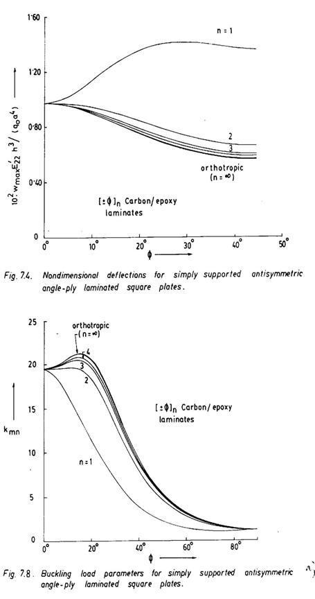
The values of maximum nondimensional deflections (at x₁=x₂=a/2) for simply supported antisymmetric angle-ply laminated square plates are plotted against the variation of Ø ranging from 0 to 45⁰. A two-layered laminate is found to exhibit much higher deflections due to higher values of coupling terms B₁₆ and B₂₆ compared to the other cases.

7.4 FREE VIBRATION AND BUCKLING

7.4.1 Specially Orthotropic Plate

Consider a rectangular specially orthotropic plate (Fig. 7.5) which is subjected to compressive loads and per unit length along the edges. The plate is also assumed to be vibrating freely in the transverse direction. Equation 7.12 then becomes (note that )

(7.52)

All Edges Simply Supported

The deflected shape w (x₁,x₂, t) is assumed in the following form:

(7.53)

that satisfies the simply supported boundary conditions in Eqs. 7.16. Substitution of Eq. 7.53 in Eq. 7.52 yields the frequency equation as follows

(7.54)

where

and . Note that is the circular frequency.

The non-dimensional frequency parameter can be computed for a particular mode shape m and n for various values of aspect ratio (a/b), stiffness ratios and inplane loads. From Eq. 7.54, it is evident that a critical combination of compressive inplane biaxial loads can reduce the frequency to zero. When the frequency is zero, the inplane loads correspond to the buckling loads of the plate. Further, it may be noted that the tensile inplane loads will increase the frequency of the plate.

Two Opposite Loaded Edges Simply Supported

For a laminated plate, where the compressive edge load acts along the simply supported edges x₁=0,a and the unloaded edges x₂=0, b may have any arbitrary boundary condition, a solution to Eq . 7.52 (note that ) can be assumed to be in the form

(7.55)

Substituting Eq. 7.55 in Eq. 7.52 yields

(7.56)

A solution to Eq. 7.56 can be obtained as follows

(7.57)

Substituting Eq. 7.57 in Eq. 7.56 we obtain

(7.58)

where

and

with

Equation 7.58 has four roots i.e., with

and

Thus the solution is

(7.59)

The coefficients A_m, B_m, C_m and D_m are determined from boundary conditions at x₂=0, b. For example, let us consider the clamped edges along x₂=0, b i.e.,

X₂=0,b: w=w_{, 2}=0 (7.60)

Combining Eqs. 7.59 and using Eqs. 7.60, we obtain the following homogeneous algebraic equations

(7.61)

The frequency equation is obtained from the condition that the determinant of the coefficients of A_m, B_m, C_m and D_m must vanish. This leads to

(7.62)

The critical value of N is computed by satisfying Eq. 7.62 for a particular m when the frequency becomes zero.

7.4.2 Antisymmetric Cross-ply Laminated Plate

Consider the transverse force vibration of a simply supported rectangular antisymmetrically laminated cross-ply plate (see section 7.3.2), when subjected to compressive loads , and . Equations 7.44 hold good except the third equation where 'q' is replaced by “ “. The following displacement field

(7.63)

satisfy the boundary conditions in Eqs. 7.45. These, on substitution in Eqs. 7.44 modified as above, result in the following homogeneous algebraic equations:

(7.64)

where

and .

The frequency relation is derived by vanishing the determinant of the coefficient matrix of Eq. 7.64 and is given by

(7.65)

wher and k_mn are defined in Eq. 7.54.

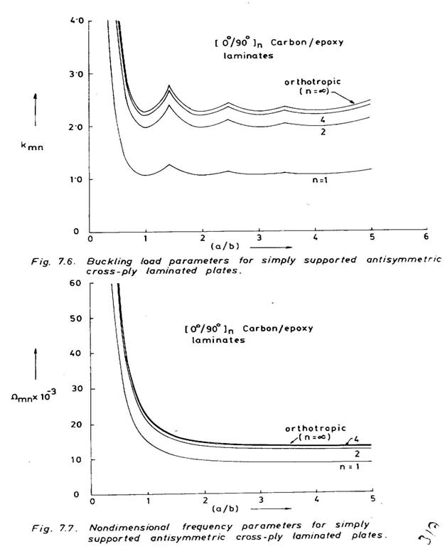
The critical buckling load corresponds to the lowest value of k that satisfies Eq. 7.65 when the frequency is zero. The load parameters, k_mn and nondimensional frequency parameters, are plotted against the aspect ratio, a/b for simply supported antisymmetric cross-ply laminate as shown in Figs. 7.6 and 7.7, respectively.

7.4.3 Antisymmetric Angle-Ply Laminated Plate

Now consider the transverse free vibration of a simply supported rectangular antisymmetric angle-ply laminated plate (vide section 7.3.3) which is subjected to compressive loads , and . The third equation in Eqs. 7.48 is modified substituting - in place of q. The displacement field that satisfies the boundary conditions in Eqs. 7.49 is assumed as

(7.66)

These displacement relations, when substituted in the modified Eqs. 7.48 yield the following homogeneous algebraic equations:

(7.67)

where

The condition that the determinant of the coefficient matrix in Eq.7.67 vanishes, determines the frequency equation as follows:

(7.68)

where

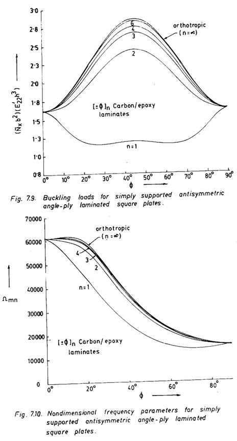
Figures 7.8 and 7.9 depict the variation of bucklin

g load parameters and Figure 7.10 shows that of the frequency parameter for simply supported antisymmetric angle-ply laminated square plates.

7.5 SHEAR BUCKLING OF COMPOSITE PLATE

A closed form solution for the shear buckling of a finite composite plate does not exist. This is true also for an isotropic panel. Here the solution of a long specially orthotropic composite plate is considered. Consider the plate to be infinite along the x₁ direction and is subjected to uniform shear along the edges x₂ = ±b/2 (Fig. 7.11). In absence of inertia and other loads except the edge shear , Eq. 7.12 becomes

(7.69)

Assuming the solution to be of the form

(7.70)

where k is a longitudinal wave parameter and . Substituting Eq. 7.70 in Eq.7.69 we obtain

(7.71)

A solution to Eq.7.71 is assumed to be of the form

(7.72)

which on substitution in Eq. 7.71 yields the following characteristic equation

(7.73)

Equation 7.73 has four roots and the solution to Eq. 7.69 is written as follows:

(7.74)

Combining Eqs. 7.70 and 7.74, the solution is obtained as

(7.75)

The substitution of Eq. 7.75 in the specified boundary conditions at the edges x₂ = ±b/2 will result four homogeneous algebraic equations in terms of the four coefficients A, B, C and D. For a non-trivial solution, the determinant of this coefficient matrix must vanish. This condition yields the equation for the shear buckling problems. The critical buckling load corresponds to the minimum value of at particular value of k.

7.6 RITZ METHOD

The Ritz method (also known as the Rayleigh-Ritz method), in most cases, leads to an approximate analytical solution unless the chosen displacement configurations satisfy all the kinematic boundary conditions and compatability conditions within the body. It is developed minimizing energy functional on the basis of energy principles. The principle of minimum potential energy can be used for formulation of static bending and buckling problems. The free vibration problem is formulated using Hamilton 's principle.

The total strain energy of a general laminated plate is given by (Fig. 7.1)

(7.76)

Substituting Eq. 6.59 in Eq . 7.76, one obtains

(7.77)

Substituting Eqs.6.47 through 6.49 in Eq. 7.77, and using Eqs. 6.53, 6.61 and 6.62 we obtain

(7.78)

The potential energy of external surface tractions and edge loads due to the deflections of the plate is given by

(7.79)

The kinetic energy of the laminated plate can be expressed as

(7.80)

where P, R, and I are defined in Eqs. 7.6.

The Ritz method can be utilized for seeking solution to a particular problem. The approximate displacement functions are chosen to be in the following form

(7.81)

where the shape functions u_1i(x₁, x₂), u_2i(x₁, x₂) and w_i(x₁, x₂) are capable of defining the actual deflection surface and satisfy individually atleast the geometric boundary conditions, and a₁, b₁, and c₁ are undetermined constants.

For the bending of a general laminated plate, the energy functions, is defined as

(7.82)

where U and V are represented in Eqs 7.78 and 7.79, respectively.

The principle of minimum potential energy leads to the following conditions.

(7.83)

that provide m + n + r simultaneous algebraic equations for the computation of m+n+r unknown coefficients a_i, b_i, and c_i.The approximate solution is thus obtained by substituting these coefficients in the assumed displacement functions in Eqs 7.81.

For the solution of plate buckling problem, only the edge loads are retained assuming , , in the expression for the potential energy V in Eqs. 7.79 and 7.82. The application of conditions in Eq. 7.83 results a set of m+n+r algebraic homogeneous equations in terms of m+n +r coefficients a_i, b_i, and c_i. The vanishing of the determinant of the coefficient matrix yields the buckling equation from which critical buckling loads are determined.

For the free vibration problem, the displacement functions in Eqs. 7.81 can be modified to include the time dependence as follows:

(7.84)

where the U₁(x₁, x₂), U₂(x₁, x₂), and W(x₁, x₂), correspond to the right-hand-side expressions in Eqs. 7.81. The energy functional П^* includes the strain energy U and kinetic energy T. Hence П^* = U+T. In the absence of surface forces and moments, edge loads and expansional stress resultants and moments, and substituting Eq. 7.84 in the above energy functional П^*and carrying out the derivation of П^*with respect to a_i, b_i, and c_iand equating them to zero i.e. , and , we obtain a set of m+n+r coefficients a_i, b_i, and c_i. The frequency equation is derived from the condition that the determinant of the coefficient matrix must vanish.

7.7 GALERKIN METHOD

The Galerkin method utilizes the governing differential equations of the problem and the principle of virtual work to formulate the variational problem. Here the virtual work of internal forces is obtained directly from the differential equations without determining the strain energy. The Galerkin method appears to be more general than the Ritz method and can be very effectively utilized to solve diverse general laminated plate bending problems involving small and large deflection theories, linear and nonlinear vibration and stability of laminated plates and so on.

Consider a general laminated plate (Fig. 7.1) to be in a state of static equilibrium under loads q_1,q₂and q only Then the governing differential equations in Eqs. 7.7 through 7.9 can be expressed as follows:

(7.85)

The equilibrium of the plate is obtained by integrating Eqs. 7.85 over the entire area of the plate. Note that, if required, the edge loads and expansional force resultants and moments can also be included in Eqs. 7.85.

Assuming small arbitrary variations of the displacement functions and applying the principle of virtual work, we obtain the variational equations as follows:

(7.86)

As in the Ritz method, we assume the approximate displacement functions in Eqs. 7.81, where the shape functions u_1i(x₁,x₂), u_2i(x₁,x₂) and w_i(x₁,x₂), satisfy the displacement boundary conditions but not necessarily the forced boundary conditions, in which case the method leads to an approximate solution.

Now,

(7.87)

Substitution of Eq. 7.87 in Eq. 7.86 yields

(7.88)

The variations of expansion coefficients are arbitary and not inter-related. This provides m+n+r equations.

(7.89)

to determine m+n+r unknown coefficients a_i, b_i, and c_i.

Note that, in a rigorous sense, the variational relations in Eqs. 7.86 are valid only, if the assumed displacement functions are the exact solutions of the problem. Thus, when these displacements are kinematically admissible and satisfy all the prescribed boundary conditions and compatibility conditions within the plate, the method leads to an exact solution.

Equations 7.85 can be used for the buckling analysis of a laminated composite plate assuming q₁= q₂=0 and replacing “q” with “” where , and . Following Eqs. 7.86 through 7.89 we obtain the variational relations of the following form:

(7.90)

Equations 7.90 are a set of m+n+r homogeneous algebraic equations in terms of m+n+r coefficients a_i, b_i, and c_i. The condition that for a non-trivial solution, the determinant of the coefficient matrix should vanish yields the buckling equation.

For the free vibration problem, the displacement functions are assumed to be of the form given in Eqs. 7.84. Considering only the transverse inertia in Eqs. 7.7 through 7.9 and neglecting surface forces and moments, edge loads and expansional stress resultants and moments, we obtain, following the procedure as in the case of buckling above, the variational relations of the form

(7.91)

These are, again, a set of m+n+r homogeneous algebraic equations in terms of m+n+r coefficients a_i, b_i, and c_i. The frequency equation is established from the condition that the determinant of the coefficient matrix must vanish so as to obtain a non-trivial solution.

7.8 THIN LAMINATED BEAM THEORY

The small deflection bending theory of thin laminated composite beams can be developed based on Bernoulli's assumptions for bending of an isotropic beam. Note that Kirchhoff's assumptions are essentially an extension of Bernoulli's assumptions to a two-dimensional plate problem. Hence the governing laminated plate equations as developed in earlier sections can be reduced to one-dimensional laminated beam equations.

Consider a thin laminated narrow beam of length L, unit width and thickness h (Fig. 7.12). The governing differential equations defined in Eqs. 77 through 7.9 reduce to the following two one-dimensional forms:

(7.92)

Consider the bending of a laminated composite shown in Fig. 7.12 under actions of transverse load q(x₁) only. Equations (7.92) assume the form

(7.93)

Consider, for example, the following simply supported boundary conditions at x₁ = 0, L:

and (7.94)

Assume the displacement functions to be of the forms

(7.95)

that satisfy the boundary conditions in Eqs. 7.94. Assume the transverse load q(x₁) as

(7.96)

Substituting Eqs. 7.95 and 7.96 in Eqs. 7.93 and carrying out the algebraic manipulation, we obtain

and (7.97)

where q_m for a particular distribution of load q(x₁) is obtained from

(7.98)

Equations 7.95 in conjunction with Eqs. 7.97 provide solution to the above beam bending problem. Note, that for a uniformly distributed transverse load q_0,

Next consider the free transverse vibration and buckling of a simply supported laminated beam. The following governing differential equations are considered (; see Eqs. 7.92):

(7.99)

The displacement functions chosen are

(7.100)

that satisfy the boundary conditions defined by Eqs. 7.94. Substituting Eqs. 7.100 in Eqs. 7.99, we obtain two algebraic homogeneous equations in terms of coefficients U_m and W_m. For a non-trivial solution, the determinant of the coefficient matrix must vanish. This yields the frequency equation to be in the form

(7.101)

Note that the critical buckling load, N_cr, corresponds to the minimum value of compressive force N for a specific mode shape m, when the frequency is zero.

It is to be mentioned that the approximate analysis methods such as the Ritz method and Galerkin method can be used to obtain solutions for laminated composite beams with various other support conditions for which closed form solutions may not be easily obtainable.

7.9 PLY STRAIN, PLY STRESS AND FIRST PLY FAILURE

Once the mid-plane displacement are determined, as discussed in the previous sections, the mid-plane strains and curvatures k₁, k₂and k₆ are determined using Eqs. 6.47 and 6.48. Next the strains for any ply located at a distance z from the mid-plane (see Fig. 6.16) are computed utilizing Eqs. 6.49. Equations 6.50 are then employed to determine the ply stresses at the same location. In some cases, it is required to determine the stresses in each ply, that correspond to the material axes x₁' and x₂' (Fig. 6.12). These are obtained using the following relations (see Eqs. A.11and A.19):

(7.102)

where m = cos Ø and n = sin Ø

In many practical design problems, the first ply failure is usually the design criterion. Once the stresses are determined in each ply of a laminate, one of the failure theories presented in section 6.14 is employed to determine the load at which any one of the laminae in the laminated structure fails first ('first ply failure'). The laminate failure, however, corresponds to the load at which the progressive failure of all plies takes place. The estimation of the laminate strength is more complex.

7.10 BIBLIOGRAPHY

S. Timoshenko and S. Woinowsky-Krieger, Theory of Plates and Shells, McGraw Hill, NY, 1959.
S. G. Lekhnitskii, Anisotropic Plates, Gordon and Breach, N.Y., 1968
L.R.Calcote, Analysis of Laminated Composite Structure, Van Nostrand Rainfold, NY, 1969.
J.E. Ashton and J.M Whitney, Theory of Laminated Plates, Technomic Publishing Co., Inc., Lancaster, 1984.
J.C. Halpin, Primer on Composite Materials: Analysis, Technomic Publishing Co., Inc., Lancaster, 1987.
J.M. Whitney, Structural Analysis of Laminated Anisotropic Plates, Technomic Publishing Co., Inc., 1987.
R.M. Jones, Mechanics of Composite Materials, McGraw Hill, NY 1975.
J.R. Vinson and T. –W, Chou, Composite Materials and their Use in Structures, Applied Science Publishers, London, 1975.
K.T. Kedward and J.M. Whitney, Design Studies, Delware Composites Design Encyclopedia, Vol.5, Technomic Publishing Co., Inc., Lancaster, 1990.
J.E. Ashton, Approximate Solutions for Unsymmetrically Laminated Plates, J. Composite Materials, 3, 1969, p. 189.

7.11 EXERCISES

1. Derive the governing differential equations as defined in Eqs.7.7, 7.8 and 7.9.

2. Determine the deflection equation for a simply supported square (axa) symmetric laminated plate subjected to a transverse load q=q₀ x₁/a.

3. Determine the deflection equation for a square (axa) symmetric laminated plate subjected to a transverse load q=q₀ x₁/a when the edges at x₁ = 0, a are simply supported and those at x₂ = 0, b are clamped.

4. A simply supported antisymmetric cross-ply laminated (0⁰/90⁰/0⁰/90⁰) kelvar/epoxy composite square plate (0.5m x 0.5m x 5mm) is subjected to a uniformly distributed load of 500N/m². Determine the deflection an dply stresses at the centre of the plate. Use properties listed in Table 6.1.

5. A simply supported antisymmetric angle-ply laminated (45⁰/-45⁰/45⁰/-45⁰) carbon/epoxy composite plate (0.75m x 0.5m x 5mm) is subjected to a uniformly distributed transverse load q₀. Determine the load at which the first ply failure occurs. Use the Tsai-Hill or Tsai-Wu strength criterion. See Table 6.1 and also assume X '₁₁^t =1450 MPa, X '₁₁^c=1080 MPa, X '₂₂^t=60 MPa,

X'₂₂^c =200 MPa and X '₁₂= 80 MPa.

6. Determine the transverse natural frequencies for the plates defined in Problems 4 and 5 above. Neglect the transverse load.

7. Determine the uniaxial compressive buckling loads for the plates defined in problem 4 and 5 above. Neglect the transverse load.

8. Make a comparative assessment between the Ritz method and the Galerkin method.