CHAPTER - 4

COMPOSITE PROPERTIES - MICROMECHANICS

4.1 INTRODUCTION

4.2 UNIDIRECTIONAL COMPOSITES

    4.2.1 Elastic Properties (Engineering Constants)

    4.2.2 Strength Properties of Unidirectional Composites

    4.2.3 Hygrothermal Properties

4.3 PARTICULATE AND SHORT FIBRE COMPOSITES

    4.3.1 Particulate Composites

    4.3.2 Short Fibre Composites

4.4 BIBLIOGRAPHY

4.5 EXERCISES

4.1 INTRODUCTION

            The mechanical and hygrothermal properties of composites are of paramount importance in the design and analysis of composite structures. The mechanical properties constitute primarily the moduli and strength properties. The hygrothermal properties are coefficient of expansion due to moisture (β), misture diffusion coefficient (d), coefficient of thermal expansion (α), thermal conductivity (k) and heat capacity (c). Micromechanical analyses concern with the theoretical prediction of these properties of constituent fibres and matrices as well as several other parameters like the shape, size and distribution of fibres, fibre misalignment, fibre-matrix interface properties, void content, fibre fracture, matrix cracking and so on. The studies in micromechanics utilize micro-models, as the fibre diameters usually vary in the microscopic scale between 5-140 µm. The micro-models should simulate the microstructure of a realistic composite, but that usually makes the models highly complex. The problems involving such complex models are normally tackled utilizing advanced analytical methods as well as numerical analysis techniques(finite element and finite difference methods). Even in the case of a complex model, a simplified idealization with a reasonably good approximation of the real composite is desirable otherwise it may lead to nowhere. It is not intended in this chapter to present the complete theoretical basis of various micro-models used for the analytical prediction of all composite properties. The presentation is limited to only a few simpler cases so as to acquaint the reader of the background of the development in this area. Additional micromechanics relations for unidirectional composites, that may find use in design applications, are listed in Table 4.1. Typical properties of some of the common fibres and matrices are listed in Tables 4.2 and 4.3, respectively. The composite properties of a few composite systems derived using some of the relations presented in this chapter are listed in Table 4.4. Tables 4.1 through 4.4 are included at the end of this chapter.

4.2 UNIDIRECTIONAL COMPOSITES

4.2.1 Elastic Properties (Engineering Constants)

            The stress-strain relation provides the basic interface between a material and a structure. For a one dimensional isotropic, elastic body, the Hooke's law σ = E  defines the stress-strain behaviour. Here E is a material constant and is usually referred as elastic constant (engineering constant) or Young's modulus. Besides E, the other conventional engineering constant for a two-dimensional or three-dimensional isotropic body is Poisson's ratio ν. The shear modulus G is not independent, but is related to E and ν as

G = E/2(1+ ν). A composite material is essentially heterogeneous in nature, therefore the engineering constants, defined above, for an isotropic material are not valid. We consider here a three-dimensional block of a unidirectional composite (Fig. 4.1), in which fibres are aligned along the x'₁ axis. The elastic behaviour for such a three-dimensional body

is orthotropic, and the engineering constants are , ,  (three Young's moduli along three principal material axes x'₁, x'₂, x'₃), ν'₁₂, ν'₁₃, ν'₂₃, ν'₂₁, ν'₃₁, ν'₃₂, (six Poisson's ratios) and G'₁₂, G'₁₃, G'₂₃, (three shear moduli). Of these, the first nine engineering constants i.e., three Young`s moduli and six Poisson ratios are not independent. Due to symmetry of compliances (see Eq. 6.18) these are related as given by

                                                                     (4.1)

Note that,

                                           (4.2)

Here ν'₁₂ and ν'₁₃ are usually referred as major Poisson ratios.

            The 'mechanics of materials approach' provides convenient means to determine the composite elastic properties. It is assumed that the composite is void free, the fibre-matrix bond is perfect, the fibres are of uniform size and shape and are spaced regularly, and the material behaviour is linear and elastic.

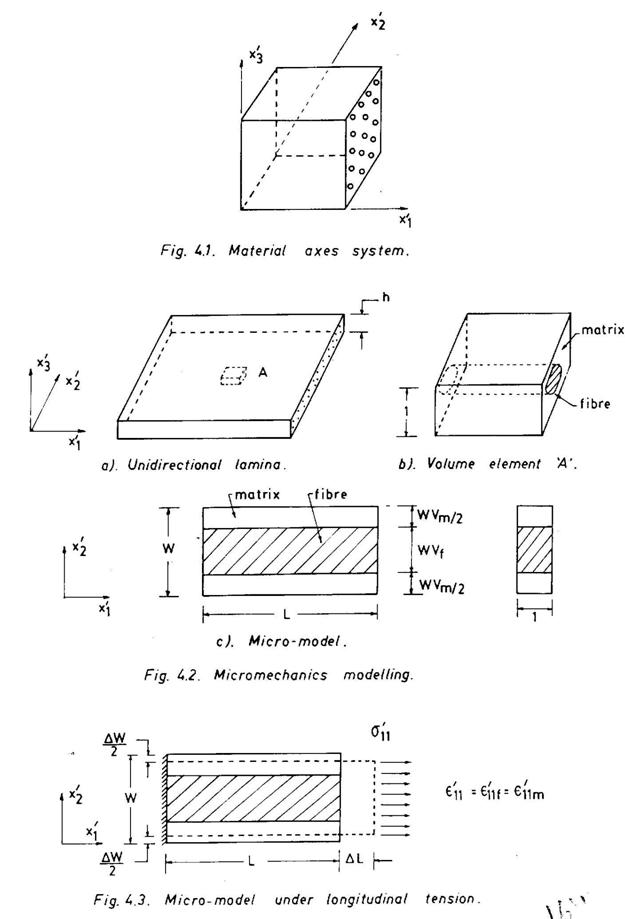
            Consider a two-dimensional unidirectional lamina (Fig. 4.2), in which we define a small volume element which represents not only the micro-level structural details but also the overall behaviour of the composite. A simple representative volume element consists of an isotropic fibre embedded in an isotropic matrix (Fig. 4.2b). This volume element is further simplified as shown in Fig.4.2c, in which the fibre is assumed to have a rectangular cross-section with the same thickness as the matrix. The width ratio is chosen to be the same as the fibre volume fraction of the composite itself. The objective is to derive the composite properties (E'₁₁, E'₂₂, ν'₁₂, G₁₂) in terms of the moduli, Poisson`s ratios and volume fractions of the fibre and the matrix.

Longitudinal modulus , E'₁₁

                The micro-model (Fig. 4.2c) is subjected to a uniaxial tensile stress σ`₁₁ as shown in Fig. 4.3. It is assumed that plane sections remain plane after deformation. Hence,

'₁₁= '_11f = '_11m  = ΔL/L

and       σ'_11f = E'_11f   '₁₁, σ'_11m =  E'_11m '₁₁, σ'₁₁ = E'₁₁  '₁₁                                           (4.3)

Now,   σ'₁₁ W = σ'_11f   W_f   +    σ'_11m   W_m                                                       (4.4)

Substituting Eq. (4.3) into Eq. (4.4) and rearranging, we have

E'₁₁ =  E'_11f W_f / W  +   E'_11m  W_m  / W                                                                                                (4.5)

Noting that the volume fractions of the fibre and the matrix are

V_f = W_f /W and V_m = W_m / W respectively, Eq. 4.5 reduces to                                   

            E'₁₁ = E'_11f  V_f   + E'_11m V_m                                                                                                                           (4.6)

Equation 4.6 defines the composite property as the 'weighted' sum of constituent properties and is often termed as the 'rule of mixture'.

 Transverse modulus, E'₂₂        

                The tensile stress σ'₂₂ is applied along the x'₂ direction (Fig. 4.4) and the same is assumed to act both on the fibre and the matrix. The strain on the fibre and the matrix are

'_{22 f}   = σ'₂₂ / E'_22f   and '_22m = σ'₂₂ / E'_22m                                                             (4.7)

also      '₂₂       =   ΔW/W

and       ΔW = '_22f    (V_f W) + '_{22 m} (V_m  W)

So,        '₂₂     =   ΔW/W  =  '_{22 f} V_f  +  '_{22 m} V_m

or,                        

or,                                            

or,                                                                                                   (4.8)

Major Poisson 's Ratio,  ν '₁₂   

             The micro-model is stressed as in the case of determination of E`₁₁ (Fig. 4.3). The transverse contraction is noted as ΔW and is contributed by both the fibre and matrix. Thus,

            ΔW = (ΔW)_f  + (ΔW)_m

or,        ΔW = W V_f  ν '_12f     '₁₁   +   W V_m ν '_12m  '₁₁                                                                (4.9)

Now ,                                                                                                       (4.10)

and        '₂₂       = - ΔW/W                                                                                             (4.11)

Combining Eqs. 4.9 through 4.11, one obtains

or,        ν '₁₂    =   V_f  ν '_12f    +   V_m  ν '_{12 m}                                                                         (4.12)

Inplane Shear Modulus, G '₁₂

            The micro-model is now subjected to a shear stress σ '₁₂ as shown in Fig. 4.5, and both and the fibre and the matrix are assumed to experience the same shear stress.

             '_12f  = σ '₁₂ / G '_12f  and   '_12m  =  σ '₁₂ / G '_12m                                                      (4.13)

Now,   Δ =  '₁₂W  =  W V_f  '_12f  + W V_m   '_12m              

or,         '₁₂  = V_f   '_12f   +  V_m  '_12m                                                                         (4.14)

also,                                                                                                             (4.15)

            Substituting Eqs. 4.13 and 4.15 into Eq. 4.14 and eliminating σ '₁₂  from both sides, we get

or,                                                                                          (4.16)

Note that, for an isotropic fiber

            E'_11f = E'_22f = E_f ,  ν'_12f  = ν_f

and                                                                                          (4.17)

and for an isotropic matrix

            E'_11m  =  E'_{22 m}   =  E_m  ,   ν'_12m  =  ν_m

and                                                                                          (4.18)

Equations 4.6 and 4.12 provide a reasonably accurate estimate of longitudinal modulus E´₁₁ and ν´₁₂, respectively. However, the transverse modulus E´₂₂ and the shear modulus G´₁₂, estimated using Eqs. 4.8 and 4.16, are not so accurate mainly due to the reason that the stresses in both the fibre and the matrix are assumed to be the same. The volume element considered in the above mechanics of materials approach does not adequately represent the micro structure of the composite. Advanced analytical methods employ better micro-models along with the realistic material behaviour and boundry conditions. The analytical method using a self-consistent field model provides a better estimation of composite properties in comparison to the ‘mechanics of materials’ approach. The model assumes the composite to be a concentric cylinder (Fig. 4.6) in which a transversely isotropic matrix. Although the assumed micro-model is simple, it permits formulation of the problem based on the theory of elasticity so that it is possible to achieve the stress and strain variations in a realistic manner, and the relations for the effective composite properties are then derived. These properties are expressed as follows:

                    (4.19)

                     (4.20)

                                       (4.21)

                  (4.22)

                                                   (4.23)

where K' is the plane strain bulk modulus.

                                                                (4.24)

in which K', G'₂₃, ν'₁₂² and E'₁₁are defined in Eqs. 4.19 through 4.23.

                                                              (4.25)

with E'₁₁, E'₂₂, K', and ν'₁₂ defined in the above relations.

Note that for isotropic fibres and matrices,

;

and                                                   (4.26)

4.2.2 Strength Properties of Unidirectional Composites

            The strength of a material is defined as the level of stress at which failure occurs. The strength is a material constant. Most of the isotropic structural materials possess only one constant i.e., the uniaxial tensile strength. The shear strength is normally related to the tensile strength. A brittle isotropic material may have different strength values in tension and compression and may be termed as a two-constant material. In contrast, a composite is a multi-constant material. Referring to Fig. 4.1, it may be stated that a unidirectional composite may possess three normal strengths X'₁₁, X'₂₂, X'₃₃ and three shear strengths X'₁₂ , X'₁₃, X'₂₃. A normal strength may have different values in tension and compression, as the compressive force usually induces premature failure due to buckling of fibres which have extremely high slenderness ratio. So there are a total of nine independent strength constants X'₁₁^t, X'₂₂^t, X'₃₃^t, X'₁₁^c, X'₂₂^c, X'₃₃^c, X'₁₂, X'_13, X'₂₃.

            Attempts made using micromechanical analyses to determine these strength constants, met with little success. This is primarily due to the reason that the micro-models used in these analyses are grossly unrealistic. In fact, it is extremely difficult to simulate the realistic composite, as the initial microstructure changes continuously with the increase of applied stress and propagation of failure in the form of fibre fracture, matrix cracking, fibre-matrix debond and so on at several points located randomly within the composite. The brittleness of the fibre and the matrix aggravates the situation. This is illustrated in Fig. 4.7. Note that l_c is the ineffective length. The presence of a single surface flaw in a brittle fibre causes the fibre to fracture at A (Fig. 4.7a). This induces high shear stresses and causes the fibre-matrix debond along the fibre direction (Fig. 4.7b). Also when a fibre fractures, a redistribution of stresses in the vicinity results in the tensile fracture of the adjacent fibre due to stress concentration. This process leads to the propagation of the crack in the direction transverse to the propagation of the crack in the direction transverse to the fibres (Fig. 4.7c). In fact, the final failure of a composite is resulted due to the cumulative damage caused by several micro and macro-level failures.

Longitudinal Tensile Strength, X'₁₁^t

            A simple relation can be derived for the longitudinal tensile composite strength X'₁₁^t using the 'rule of mixtures' and is expressed as

X'₁₁^t = X'_11f V_f   + X'_11m V_m                                                                               (4.27)

Here it is assumed that, at a particular level of stress, all fibres fracture at the same time and the failure occurs in the same plane. That this idealization is grossly unrealistic has already been argued in the preceding paragraph.

            Now, let us examine the validity of Eq. 4.27 for two composite systems: (i) a carbon/epoxy composite, in which the fibre failure strain is less than the matrix failure strain, i.e., '_11fu < '_11mu (Fig. 4.8a) and (ii) carbon/carbon composite when '_11fu > '_11mu (Fig.4.8b). In these cases, both fibres and matrices are brittle. In the case of carbon/epoxy composite, when V_f is much higher than V_m , the strength of the composite is primarily controlled by the fibre fracture. Once the fibres fail, very little resistance is offered by the matrix. So, the strength of the composite is given by

X'₁₁^t = X'_11f  V '_f  + σ '_11m  V_m                                                                            (4.28)

where σ '_11m is the stress level in the matrix when the fibres fracture. On the other hand, when V_f  is low, there is a sufficient amount of matrix to resist the load after the failure of fibres. In that case,

X'₁₁^t   =  X'_11m^t V_m                                                                                            (4.29)

It is therefore obvious that there exists a limiting value of V_f at which the final failure changes from the fibre failure mode to the matrix failure mode. One may argue in a similar way to identify the possible failure mechanisms in the case of a carbon/carbon composite also (Fig. 4.8b) as well as in the cases of other composites in which either fibres or matrices or both are ductile. But the fact remains that there is no single relation which is able to define the uniaxial tensile strength of a realistic composite.

            However, Rosen's model of cumulative damage, which is based on the Weibull distribution of the strength-length relationship, provides somewhat better estimation of X'₁₁^t, when the fibres and the matrix exhibit brittle behaviour. This model assumes that the composite consists of N fibres of original length L and the weaker fibres fracture due to the applied tensile stress (Fig. 4.9). The original length is then divided into M segments, where each segment (bundle or link) is of length 1_c. Thus the composite forms a chain of M bundles (links). When the number of fibres are very large (high V_f) the strength of each bundle or chain link assumes the same value, i.e., the strength of the composite becomes equal to the link strength. This is expressed as 

                                                                       (4.30)

where α and β are material constants and can be determined experimentally. The tensile strength of the composite is then determined using

                                                                    (4.31)

Note that l_c is called the ineffective length or critical fibre length and is determined using the shear lag stress. It is given by

                                                                                                        (4.32)

where X'_f is the tensile fracture strength of the fibre, d is the diameter of the fibre and X_i is the fibre-matrix interfacial shear strength.

            The longitudinal compressive strength X'₁₁^c of a unidirectional composite is primarily affected by the buckling of fibres. In a simplified model, the fibres are treated as isotropic thin plates lying in the x'₁ x'₂ plane (Fig. 4.10) and are supported on an isotrpic elastic medium (matrix). Fibres may buckle in two modes-extension and shear. In

the extension mode, the matrix along the length of the fibre experiences alternate expansion and contraction, whereas the matrix is subjected to shearing deformation in the shear mode. The compressive strength is then determined employing the strain energy method. For the extensional mode,

                                                 (4.33)

or,                                                              (4.34)                                                                                                    

and for the shear mode

                                                                                                (4.35)

            The transverse strength properties normally depend on the matrix properties. The transverse tensile strength X'₂₂^t may also depend on the fibre-matrix interface strength, as illustrated in Fig. 4.11. The experimental data for some composites confirm that the transverse tensile strength enhances with the improvement in the fibre-matrix interface bond. The actual fracture path, however, is a mixture of fibre-matrix debond, fibre splitting and matrix cracking. A realistic model should be based on the variation of statistical data for all these failure modes. Two simple relations, for the prediction of the transverse tensile strength X'₂₂^t and transverse compressive strength X'₂₂^c of a unidirectional composite, are presented as follows:

                                                      (4.36)

                                                      (4.37)

These relations assume that the transverse strength of a composite primarily depends on the strength of the matrix.

4.2.3 Hygrothermal Properties

Transport Properties

            The evaluation of transport properties like moisture diffusivity, heat conductivity, electric conductivity, dielectric constant and magnetic permeability of a unidirectional composite follows the similar procedure when one uses a self-consistent field model. The resulting relations are, therefore, identical for all transport properties. The procedure is, hence, illustrated considering only one case – the diffusion of moisture through a unidirectional composite. Consider the concentric cylindrical model as shown in Fig. 4.6. Both the fibre and the matrix are assumed to be moisture permeable. For example, aramid fibres and polymer matrices are moisture permeable. For the diffusion of moisture along the fibre direction (x'₁ axis), the moisture diffusion equation assumes the form

                                                                                                 (4.38)

where C is the moisture concentration per unit volume, t is time and d'₁₁ is the longitudinal moisture diffusion coefficient of the composite.

Steady state condition

Equation 4.38 takes the form

                                                                                  (4.39)

Assuming the boundary conditions (Fig. 4.6) to be as at

x'₁ = 0, C = 0 and x'₁ = L, C = C₀                                                                     (4.40)

the solution is derived as

                                                                                                       (4.41)

that satisfies Eqs. 4.39 and 4.40.

            The direction of moisture diffusion per unit area parallel to the x'₁ direction is defined as

                                                                              (4.42)

            The total rate of moisture diffusing through the cross-section of the concentric cylinder is given by

                                                          (4.43)

Note that

and                                                                                 (4.44)

where d'_11f and d'_11m  are the longitudinal moisture diffusivities for the fibre and the matrix, respectively. Substituting Eqs. 4.42 and 4.44 in Eq. 4.43 and noting that

R_f²/R² = V_f and (R² - R_f²) / R² = V_m  one obtains

d'₁₁  =  d '_11f  V_f    +   d'_11m  V_m                                                                                        (4.45)

when the fibres (e.g., glass, carbon, etc.) are impermeable to moisture

d'₁₁  =   d '_11m  V_m                                                                                                                         (4.46)

            The transverse moisture diffusion coefficient d '₂₂ can also be determined using a similar self-consistent field model and is, given as

                                                             (4.47)

When fibres are impermeable to moisture, Eq. 4.47 reduces to

                                                                                            (4.48)

            The longitudinal and transverse thermal conductivities k'₁₁ and k'₂₂ of the unidirectional composite can be determined by replacing 'd ' with 'k' in Eqs.4.45 and 4.47, respectively. Note that, in that case, heat conduction takes place both through the fibre and the matrix. The other transport properties can also be derived in a similar way using Eqs. 4.45 and 4.47.

Expansional Strains

            The longitudinal expansional strains (due to temperature or moisture) of a unidirectional composite can be determined using the simple 'mechanics of materials approach ' as discussed earlier. Consider the micro-model in Fig. 4.3. The total longitudinal strains, after accounting for the mechanical strain and the expansional strain, are given as

and also    and also                                       (4.49)

Solving Eqs. (4.49) one gets

and                                             (4.50)

Assuming free expansion '₁₁ =  '₁₁^e, the first relation of Eqs. 4.50 yields

            σ '₁₁ = 0                                                                                                            (4.51)

Therefore,

σ '₁₁ W = σ '_11f  W_f   + σ '_11m  W_m  = 0             

   or,                                                              (4.52)

Dividing Eq. (4.52) by W and noting that  and and

V_m  = W_m / W one obtains

                                                                 (4.53)

            Observing that the thermal expansional strain of a specimen of length L due to a rise of temperature ΔT is given by ^e = LαΔT, the longitudinal thermal expansion coefficient α'₁₁ of a unidirectional composite is derived from Eq. 4.53 as follows:

                                                                     (4.54)

Similarly, the longitudinal moisture expansion coefficient β'₁₁ of a unidirectional composite is obtained from Eq. 4.54 replacing 'α' by 'β'.

            For the transverse expansional strain '₂₂^e, the 'self-consistent field model ' approach is, however, preferred. The expression for '₂₂^e can be derived as

                                 (4.55)

The transverse thermal expansion coefficient α'₂₂ is then derived from Eq, 4.55 in a similar way

                            (4.56)

The transverse moisture expansion coefficient β'₂₂ is obtained from Eq. (4.56) by replacing 'α' with 'β'.

4.3 PARTICULATE AND SHORT FIBRE COMPOSITES

            A unidirectional composite provides some sort of regularity in the microstructure, as the fibres are continuous and aligned in one direction. This helps to assure a simple micro-model with a constant strain or stress field and use the 'mechanics of materials ' approach to determine the composite properties. Such a simple analytical treatment with constant stress or constant strain field is not adequate in the case of particulate and short fibre composites. The microstructure is not uniform through the composite medium. The point to point variation of the microstructure is quite significant in many situations due to wide variations in the shape, size and properties of fillers and reinforcements and their orientation and distribution in the matrix phase. The discontinuous nature of some of these reinforcements adds to more complexities. There exist innumerable high stress zones around irregular shaped particulate reinforcements and at the tips of short fibres. The assumption of constant stress and strain fields is no more valid. Further complications arise due to the anisotropy caused by the alignment of short fibres and flake particulates.

            All these preclude a general treatment of the problem. A single composite micro-model, in no way can represent all composites of this category. Composites with different reinforcements may require different micro-models and analytical treatments. This is probably the main reason why the micromechanics analysis of this class of composites has not received much attention from researchers. There is also another important reason for the dearth of information in the area. In comparison to particulate and short fibre composites, unidirectional composites find extensive uses in structural components in several engineering disciplines. This has created more awareness and, in turn contributed to the growth of knowledge in the micromechanics of unidirectional composites, while the understanding of the micromechanical behaviour of particulate and short fibre composite still continues to remain at its nascent stage.

4.3.1 Particulate Composites

            The simplest mechanics of materials approach uses classical Voigt (constant strain) and Reuss (constant stress) models to estimate the elastic properties for an isotropic composite. With the Voigt model, the bulk modulus k and the shear modulus G are given as

P= V_f  P_f   +  V_m P_m ,                            

           where P=K,G                 

           and E = 9 KG / (3K+G)

ν = (3K-2G) / (6K+2G)                                                                                   (4.58)

and with the Reuss model, the relations are

                                                                              (4.59)

The properties predicted by Voigt model (highest) and Reuss model (lowest) are two extremes to the real values. Several improved analytical models are known to exist, but are not easily amenable to simple design uses. The Halpin-Tsai model, which is based on a semi-empirical approach, is popular and provides both upper and lower bounds that fall within the Voigt and Reuss limits. Simple relations that are developed based on an improved combining rule are found to provide a reasonably good estimate of the properties of an isotropic composite (P_f  > P_m  and 0 < ν_f  < 0.5).

            These are presented as follows:

                                                 (4.60)

with P = K,G.

For bulk modulus,                                                                             

and for shear modulus, G:                                                                       (4.61)

           Young 's modulus E and Poisson 's ratio ν are then determined from Eqs.4.60 and 4.61 using Eqs.4.58.

            The thermal expansion coefficient α is given by

                            (4.62)

where K is obtained using Eqs.4.60 and 4.61.

4.3.2 Short Fibre Composites

             A simple model assumes a randomly oriented short fibre composite as a quasi-isotropic micro-laminate in which each lamina consists of a group of short fibres oriented along a particular direction. P’ is determined using the modified Halpin-Tsai relation as given by

                                                                   (4.63)

where for

E '₁₁, longitudinal modulus, ξ = 2l / D

            E '₂₂, transverse modulus, ξ  = 2

            G '₁₂, inplane shear modulus, ξ =1

            G '₂₃, transverse shear modulus, ξ = (3 – 4 ν_m)^-1

Note, that l and d are the length and the diameter of the short fibre, respectively. Both the matrix and the fibre are isotropic in nature. The Poisson 's ratio ν'₁₂ is estimated using the simple mixture rule.

            The longitudinal tensile strength is dependent on the critical fibre length l_c (Eq. 4.32) and is given by

where σ '_m  is the stress on the matrix when the fibre breaks.

Table 4.1 Additional micromechanics relations for unidirectional composites   

1. Volume fractions:

      V_f  + V_m  + V_v =1                                                                                 (1)

      For a void free composite, V_v  = 0; V_f  + V_m  = 1 

2. Mass fractions

      M_f  + M_m  = 1                                                                                      (2)

3. Void volume fraction ρ                                                            

V_v  =  1 - ρ[ (M_f  / ρ_f ) + (M_m / ρ_m) ]                                                     (3)

4. Composite density

      ρ= ρ_f V_f  + ρ_mV_m                                                                                                             (4)

5. Fibre volume fraction 

                                                        (5)

6. Matrix volume fraction

                                                      (6)

7.   Transverse modulus

                                                 (7)

      8.   Shear moduli

                                                       (8a)

                                                                   (8b)

9.   Poisson's ratio

                                                      (9)

     10.  Longitudinal compression strength

               (fibre crushing)                                                           (10a)

                   (microbuckling)             (10b)

                                                                                                (10c)

11.       Transverse thermal conductivity

                                    (11a)

                             (11b)

            where   K_mf = 2(K_m/K_f -1)  for a cylindrical fibre.

             (for MMCs)                 (11c)

12.       Transverse moisture diffusivity

                                                                                 (12a)

            )         

                                      (12b)

where d_mf =2 (d_m /d_f -1)   for a cylindrical fibre.

13.       Thermal expansion coefficients

                                                                        (13a)

                              (13b)

                    (13c)

              (for MMCs)

                                                                                                                        (13d)

14.       Transverse moisture expansion coefficients

                                    (14)

15.       Heat capacity

                                                                            (15)

Table 4.2: Typical properties of some common fibres

Table 4.3 : Typical properties of some common matrices

Table 4.4 : Thermoelastic properties of three unidirectional composites (V_f = 0.6)

* Eqs. Of Table 4.1

4.4 BIBLIOGRAPHY

1. J.M. Whitney and R.L. McCromechanical Materials Modeling, Delware Composites Design Encyclopedia, Vol.2, Technomic Publishing Co., Inc., Lancaster, 1990.

2.  J.W. Weeton, D.M. Peters and K.L. Thomas (Eds.), Engineer's Guide to Composite Materials, American Society of Metals, Metals Park,Ohio, 1987.

3. G.S. Springer and S.W. Tsai, Thermal Conductivities of Unidirectional Material, J.Composotie Materials, 1,1967,166.

4. M. Taya and R. Arsenault, Metal Matrix Composite. Pergamon, Oxford, 1989.

5. R.A. Schapery, Thermal Expansion Coefficient of Composite Materials Based on Energy Principles, J.Composite Materials, 2, 1968,157.

6. R.M. Jones, Mechanics of Composite Materials, McGraw Hill Book Companym New York, 1975.

7. S.W. Tsai and H.T. Hahn, Introduction to Composite Materials, Technomic Publishing co., Inc., Lancaster, 1980.

8. B.D. Agarwal and L.J. Broutman, Analysis and Performance of Fiber Composites, Wiley-Interscience, NY, 1980.

9. J.C. Halpin, Primer on Composite Materials : Analysis, Technomic Publishing Co. Inc., Lancaster,1984.

10.   Z. Hashin, Theory of Fibre Reinforced Materials, NASA CR-1974, 1972.

4.5 EXERCISES

(Use material properties and formulae given in this chapter for numerical results)

1.  Using simple rules of mixture, derive expressions for E'₁₁, E'₂₂ , ν'₁₂  and G'₁₂.

2.   For a matrix of given weight, what should the weight of fibres so that the fibre volume fraction of the composite is 0.7 i.e., V_f = 0.7.

3.   For a boron/ polyimide composite (V_f = 0.7) determine the values of E'₂₂ and G'₂₂ using various formulae and make a comparative analysis.

4.   For a carbon/aluminium composite (V_f = 0.5) determine the values of E'₁₁, E'₂₂ , ν'₁₂  and G'₁₂.

5.   Determine d '₁₁ and d '₂₂ for a carbon/epoxy composites (V_f = 0.7) and for Kevlar/epoxy composite (V_f = 0.6 and d_f = 5 d_m).

6.   Determine k '₁₁ and k '₂₂ for a carbon polyimide and boron/polyimide composites (V_f = 0.7).

7.   Determine α'₁₁ and α'₂₂ for a boron/aluminium composite (V_f = 0.5).

8.   Determine β'₁₁ and β'₂₂ for a Kevlar/epoxy composite (V_f = 0.7). Assume β'_f = 0.5 β'_m.